The “Butterfish Smackdown” V. A movie of the model

Hindcast of butterfish habitat for Fall of 2010 based on the statistical model we built with the fisherman.  Hot colors are located in areas where environmental conditions are favored by the animals while cool colors (blue) occur where the model predicts conditions are unfavorable. The grey lines on the plots show isobaths where depths are 160 feet (50M)  and 660 feet (200M). You can see the habitat pour out off the Gulf of Maine in the early fall and shift south along the canyons at the edge of the continental shelf toward Hattaras.  I can imagine the butterfish chasing their own habitat as it moves south.

Today, we met over the phone for the second time with Lars Axellson and several other fisherman involved in our project.  We sent them the weblink of the movie of the model “hindcast” for fall 2010 above, as well as a description of the environmental variables that go into it .  They thought we had modeled the movement of fishing fleet….”No, no we modeled the fish” we said.  That at least suggests that our model represents a pretty good hypothesis about the features of the coastal ocean that broadly define the habitat of butterfish and probably other species including squid.   We’ll only know how accurate it is however, when we do the field evaluation.   In the end our goal is to build a model accurate enough that it allows the fisherman to avoid butterfish while fishing for squid.


What variables are in the model?:



1) A frontal index made by dividing a map of the strength of fronts (gradients) on the surface of the ocean by the distance to the nearest front of a threshold strength. The strength of fronts is based on the classification of 3 types of satellite ocean color data including those used to measure surface temperature and chlorophyll A from space.  Fronts are important concentrating structures in the ocean where feeding and other interactions between marine organisms occur.

Gradient strengths and distances to frontal gradients used to construct the gradient strength/distance frontal index map on the right.

2) A map made of an index of surface water divergence using high frequency radar measurements of surface currents.  This index describes how often the water is moving up or down above a certain threshold velocity.  The map below shows areas where water may be bringing nutrients to the surface (+) and areas where the water is converging and going downward (-). Nutrients brought to the surface in divergences should, in some places, fuel phytoplankton blooms which may then drift downstream on currents toward convergences and other kinds of concentrating surface fronts.

Map of surface current divergence.  Values greater than 0 indicate locations where the water is going up, while negative values indicate where it is going down.

3)  Sea surface temperature. In the  model we have stated that the number of butterfish is dependent on temperature but it is conditional on daylength.  For some reason that I don't understand, this SST x daylength interaction this captures seasonal migrations better than an interaction of depth by daylength.  We do see in the data that the fish can be in the nearshore and well offshore but absent in the midshelf during certain times of year.  This complicates the signal.  We have included daylength instead of day of the year because fish don't carry calenders. Daylength or "photoperiod" generally sets the biological clocks of animals, and the schedules of important life history processes like spawning.

Sea Surface Temperature.  Degrees C

4) Depth

Depth in meters

4)  The length of day in hours between nautical twilight at dawn and dusk.  This helps capture seasonal changes in habitat and often acts as a switch triggering changes  in the animals schedule of life history events as described above.  

Length of the daylight period between morning and evening nautical twilight in hours.  This changes every day.

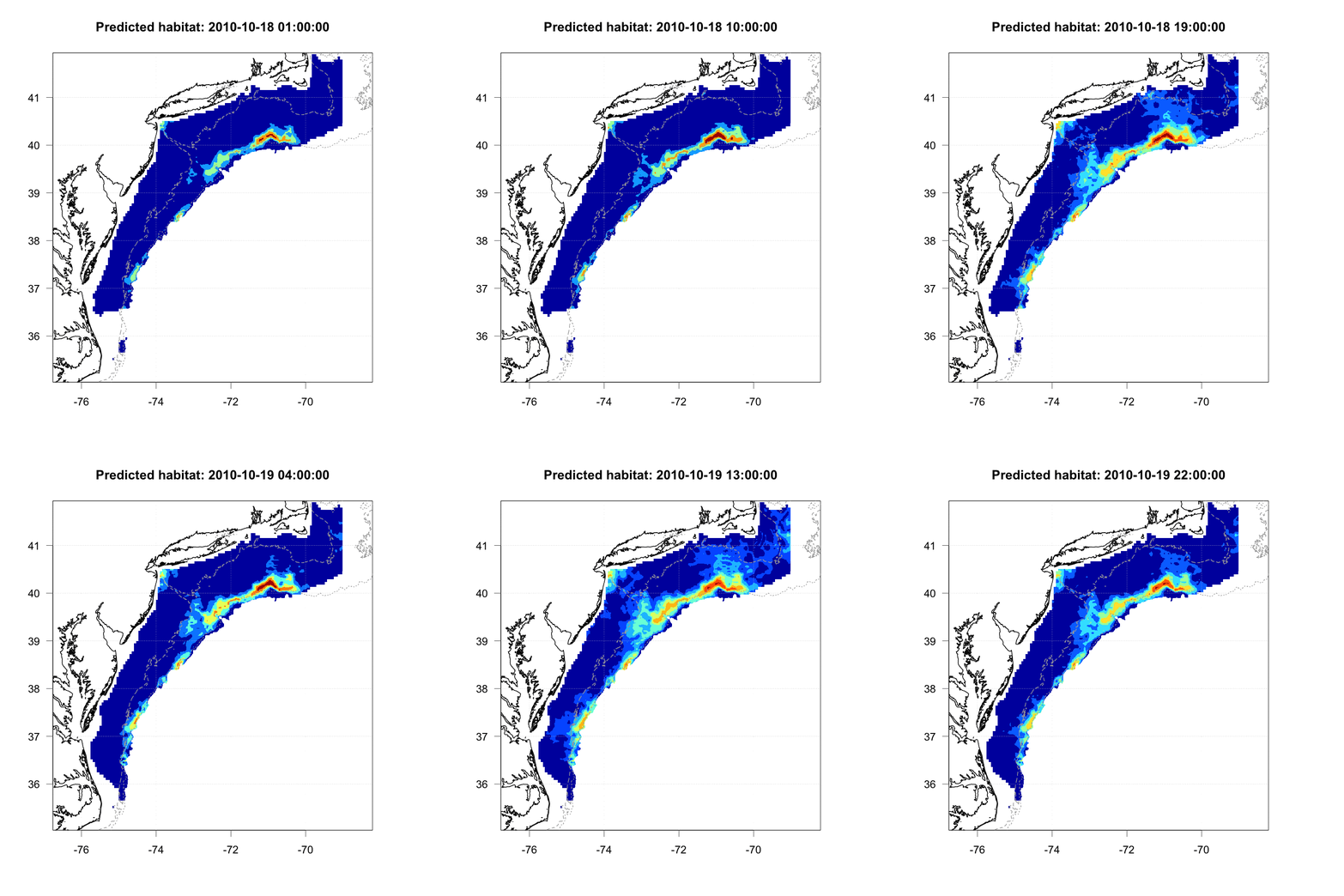
5)  The suns elevation.  This can changes hourly in the model.  The elevation of the sun seems capture the daily vertical migrations of butterfish as described in the post just below.  The effect is not location dependent in our  model so the fish are off the bottom during a period of night everywhere in the same way, and on the bottom when the sun is about 20 degrees above the horizon. The function at the top of the last post below determines the "behavior"  of the virtual butterfish in our model.  This is behavior is also shown in the movie immediately below.  Based on our conversations with Lars and the other fisherman today, vertical migration may be dependent on location and the amount of moonlight. It's probably impossible to model this level of realism. In most cases we want to make the simplest model that tries to capture the essential details.   Vertical migration could be location and time dependent if butterfish are changing their behavior based on the activities of specific predator and prey combinations. 

Sun's elevation above the horizon in degrees.  This changes hourly in the model

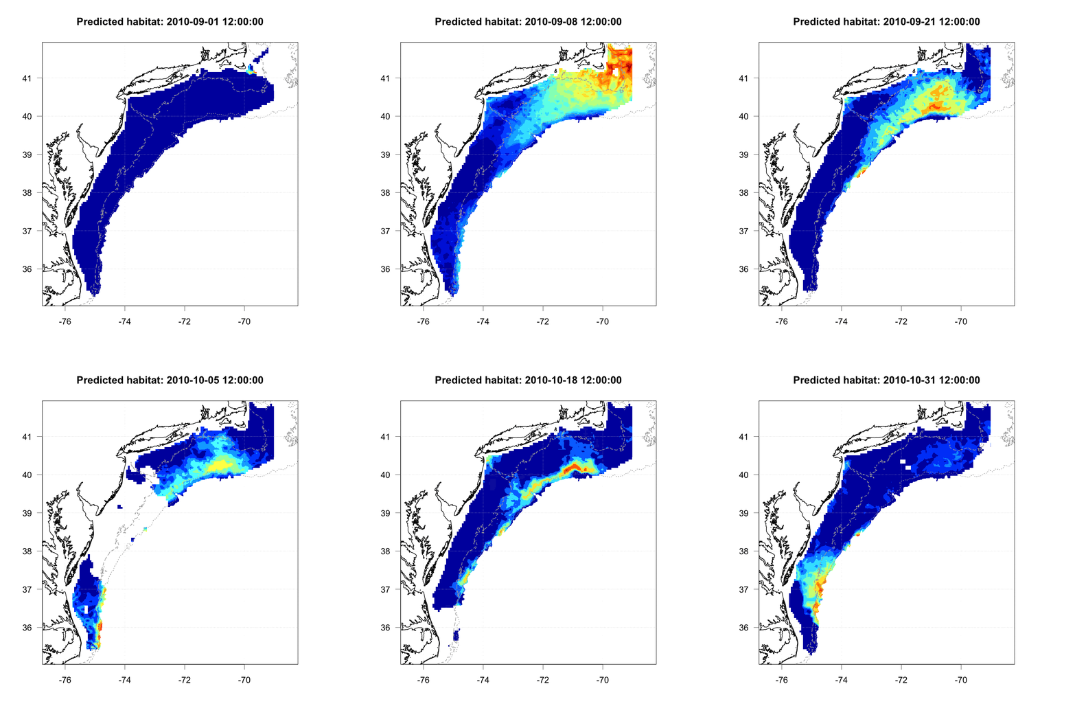
Hindcast of butterfish habitat for 2 days in the fall of 2010 with the effects of solar elevation turned on in the model we built with the fisherman. Times are in Greenwich Mean Time. Hot colors are located in areas where environmental conditions are favored by the animals while cool colors (blue) are occur where conditions are unfavorable. The grey lines on the plots show isobaths where depths are 160 feet (50M)  and 660 feet (200M). The model depicts bottom habitat. When the surface area shrinks and habitat colors cool in a location the virtual butterfish are up in the water column.