OpenOcean 2013. Does our habitat paradigm cross the land-sea boundary? A call for the development of IOOS informed seascape ecology supporting ecosystem management

John P. Manderson¹ and Josh T. Kohut²

The co-authors contributed equally to the development of this white paper submitted for 2012 National Workshops for Habitat Assessment (09/05/12) & Integrated Ocean Observation Systems (11/13/12)

¹NOAA/NMFS/NEFSC James J. Howard Laboratory, Highlands, NJ 07732

²Rutgers, The State University of New Jersey, New Brunswick, NJ 08901

“..comparison of marine and terrestrial dynamics has more than theoretical interest. As we utilize marine and terrestrial environments, the consequences, deliberate or accidental, depend on [ecosystem] responses to physical and chemical change. The imposition of terrestrial standards for marine problems may produce too strict or too lax criteria--or most likely quite inappropriate ones” (John Steele, 1991. Can ecological theory cross the land-sea boundary?)

1. Introduction

            Ecosystem assessment and management in the sea is holistic, based upon interdisciplinary science that considers physical, chemical and biological processes, including feedbacks with human ecological systems, that structure and regulate marine ecosystems.  Space and time based tools for the management of human activities in the sea need to be informed by a regional scale habitat ecology that reflects the dynamic realities of the ocean.  Current spatial management strategies including marine spatial planning (MSP) and ocean zoning are based upon the patch-mosaic paradigm of terrestrial landscape ecology modified to consider principles of dispersal ecology, primarily for pelagic early life history stages of algae, fish and invertebrates.  This modification is not enough because fundamental differences in the role fluid properties and processes play in controlling ecological processes on land and in the sea makes blanket application of paradigms developed on land to the problems of ocean management fundamentally flawed.

  The rapid evolution of the Integrated Ocean Observation System (IOOS) made possible through interdisciplinary partnerships and networked data sharing provides descriptions of coastal ocean hydrography and hydrodynamics at fine scales of space and time and regional spatial extents.  This allows hydrography and hydrodynamics to be placed at the foundation of a seascape ecology in the way that geography and geophysics appropriately serve as the foundation of terrestrial landscape ecology.   IOOS not only provides the ocean data required to develop seascape ecology but also the infrastructure and expertise to operationalize it for regional ecosystem assessment and adaptive co-management. Finally, regional IOOS associations are cooperative partnerships of academic, government and private industry experts from diverse fields and interests. As a result the IOOS "culture" can foster the collaborative development of an interdisciplinary seascape science that is more likely to lead to effective and less adversarial strategies of regional ecosystem co-management that operate at space-time scales more closely matching those of the ecosystem itself.

2. Seascapes are not landscapes

            In 1984 Paul Risser and colleagues (Risser et al, 1984) summarized workshop deliberations to develop a modern framework for the science of landscape ecology using theoretical and empirical underpinnings of a broad scale spatially explicit ecology useful for terrestrial resource management.  The foundations of this synthesis rested on (1) developments in satellite remote sensing that allowed researchers to place fine scale ecological studies in broader spatial contexts; (2) advances in ecological theory that elucidated the role of dispersal and connectivity in determining regional community dynamics; and (3) the advent of modern computing that allowed researchers to store, analyze, and model large amounts of spatially and temporally explicit data and explore relationships between the changing landscape patterns and the processes potentially causing them.  Landscape ecology rests primarily upon the patch mosaic paradigm of habitat in which patches are defined by sharp gradients in vegetation and geomorphology (but see Cushman et al. 2010).  Geography and geological processes, particularly soil development, that control fundamental processes including primary productivity are the foundations of landscape classification. In terrestrial ecosystems, most organisms and processes are decoupled from the atmosphere by gravity and physiological adaptation to extreme variations in atmospheric properties, including temperature.  As a result, the primary features of terrestrial habitats and ecosystems are physical structures created by landform and plant communities that can be modified by disturbance. Community compositions are determined by climate (Wiens, 2007).  However, the role of the atmospheric fluid is of secondary importance and the space-time scales of terrestrial ecosystems [~ velocity, 0.1 cm sec^-1] are orders of magnitude slower than the atmosphere [100 cm sec^-1] and approximately the same speed as soil regeneration (Steele, 1991; Mamayev, 1996. Fig 1).

Figure 1. Ecosystems on land (above) operate at space-time scales orders of magnitude slower than turbulent features of the atmosphere while variability in marine ecosystems (below) matches the scales of variability of turbulence in the ocean fluid.  (From Steele, 1991 and Mamayev, 1996)

In contrast, the ocean is highly viscous and has a density close to that of living tissues.  Most marine organisms are therefore nearly buoyant in a fluid with dynamics that control their motions and those of other important particles including essential ecosystem building blocks.  Since the basic processes of cellular metabolism evolved in the sea, most living tissues are nearly isosmotic with seawater. This contrasts starkly with terrestrial organisms whose intracellular concentrations of solutes and water are dramatically different than the atmosphere.  Finally the specific heat capacity and thermal conductivity of seawater are about four and twenty-three times that of atmosphere by weight, respectively.  As a result, marine organisms experience much slower rates and ranges of temperature change than do terrestrial organisms. Temperature is tyrannical in the oceans where oxygen required for endothermic heat generation is limited and warm-blooded organisms are rare. Temperature regulates critical rates across all levels of ecological organization from the cell to marine ecosystems.

            Processes controlling primary productivity on land and the sea are also fundamentally different.  In the oceans nutrients required by plants constant fall out of sunlit surface waters where photosynthesis is possible.  As a result, tiny, fast living plants with high surface to volume ratios are entirely dependent on the oceans “plumbing” to deliver nutrients into the sunlit surface layers from sometimes remote land or deep waters sources. Phytoplankton have fast population dynamics to which other members of marine food webs must respond. In contrast, primary productivity on land depends on slow, local nutrient regeneration in soil at the interface with a nearly transparent atmosphere where sunlight is rarely in short supply.   As a result, plants at the base of terrestrial food web are often immobile, long lived, and have slow population dynamics to which higher trophic levels respond.

             Due to the tight coupling of physiology, movement of organisms and other critical ecological processes to the oceans fluid, the fluid is the primary driver structuring seascapes and regulating seascape processes. As a result, ecological processes in the ocean operate at approximately the same space-time scales (~velocities [~1 cm sec^-1]) as ocean turbulence (Steele 1991, & Mamayev, 1996).  Bottom features are important to some marine organisms. However the functional importance of bottom features as surfaces concentrating advected materials, sites of energy acquisition and/or conservation in the contexts of  fluid flows, predation refugia in regions where preference for water properties such as temperature, salinity and oxygen are shared between predator and prey; are frequently primarily defined by fluid processes and properties.  

In summary, differences in the nature of the ocean and atmospheric fluid and adaptations of organisms to those fluids produce at least two critical differences in the characteristics of seascapes and landscapes.  Firstly, habitats in the sea have much faster spatial dynamics: their locations, volumes and quality change quickly at rates defined by the space-time scales of organisms responses to highly dynamic properties and processes of the oceans fluid that are driven in turn by atmospheric and planetary forcing in the form of percipiation, wind, temperature and tides. Secondly, because the ocean fluid is so viscous, horizontal and vertical currents driven by atmospheric and planetary forcing, transport essential habitat resources from sometimes remote sources and concentrate them in particular areas and times. In such cases habitats are not just locations in space supported by local resources, but nodes of networked resources and processes many of which are derived from distant "upstream" sources .  For these and other reasons relationships between habitat dynamics and processes regulating populations, including density dependent processes, are fundamentally different in the sea and on land.   Differences in the nature of habitat in the ocean and on land are in fact responsible for the order of magnitude differences in rates of change in species distribution and abundance in the sea and on land (~10 km yr^-1 vs ~ 1 km yr^-1) associated with recent rapid changes in climate (Chueng et al., 2009; Sorte et al., 2010).

3. The role of IOOS in seascape ecology 

            The presence of Integrated Ocean Observation Systems IOOS, including its infrastructure, data, models and the expertise of its diverse partners, now allows for the development of seascape ecology with a regional spatial scope that reflects the realities of the ocean.  Like landscape ecology's modern synthesis (Risser, 1984), an IOOS informed seascape ecology could provide the theoretical and empirical underpinnings for the broad scale spatially and temporally explicit ecology required for the regional assessment and management of ocean resources.   Seascape science will integrate the fields of fisheries oceanography, marine habitat ecology, and ecosystem science with hydrography and hydrodynamics at its foundation, just as terrestrial landscape ecology rests appropriately on the foundation of geography and geophysics.

 

4. Toward an IOOS informed seascape ecology

            With the support of the NOAA office of Science and Technology and North East Fisheries Science Center Cooperative Research Program we have taken advantage of the IOOS collaborative culture to form an interdisciplinary workgroup of habitat scientists, oceanographers, fishery managers, social scientists, and fishermen from academia, government and industry to develop ecologically informed habitat models for the purpose of addressing issues of related to the dynamics and assessment of habitats and populations of butterfish (Peprilus triacanthus) and longfin squid (Doryteuthis pealeii) fishery.  We held workshops to combine scientists’ and fishermen’s knowledge into a single model of butterfish habitat made using National Marine Fisheries Service (NOAA/NMFS) surveys of organisms and hydrography, and  satellite and high-frequency radar measurements of ocean properties and processes provided by the Mid-Atlantic Regional Association Coastal Ocean Observing System (MARACOOS), a regional component of IOOS (Manderson et al., 2011).  During the workshops scientists and fishermen each made “mental models” that included environmental variables each group considered important in defining habitat. Over lunch the two models were constructed and evaluated using cross-validation in a butterfish "smackdown".  Following lunch we discussed results of the “smackdown” and the ecological mechanisms potentially responsible for habitat associations described by scientists and fishermen.  Following the workshops we developed the model that combined the ecological expertise of fisherman and scientists.

            Once the combined model was complete, we worked with fishing industry partners to design an at-sea model evaluation using dynamic habitat model nowcasts provided by MARACOOS.  The combined model was adjusted slightly to include variables that has slow spatial dynamics (seabed rugosity) and fast dynamics (Sea surface temperature, water mass frontal boundaries) that could be delivered in real-time by the ocean observing system.

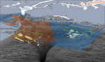
Figure 2.  Butterfish habitat preference predicted by the model during our 8-day evaluation.  The warmer colors indicate areas of preferred habitat.  The vessel track is shown in green.  

            During an 8-day trip on the F/V Karen Elizabeth, captained by Chris Roebuck, we transmitted updated dynamic butterfish habitat model nowcasts to the vessel (Fig 2). Our survey design involved sampling areas the nowcasts predicted “habitat suitability” would be  “high” and “low”. In each 3 station set we also included a site where the fisherman, Captain Roebuck, predicted butterfish would be abundant.  We sampled station sets for fish and the environment during the day and night in three canyon hotspots identified by the model along the edge of the Mid Atlantic Bight continental shelf. Using this approach we were able to formally incorporate fishermen’s knowledge into the design of our field evaluation survey. Throughout the evaluation the crew on board the Karen Elizabeth sent reports of preliminary results back to shore which we published on an online blog.

            The evaluation survey showed us that the combined model could be used to identify regions and times when butterfish concentrations were likely to be high at scales of 10s of kilometers.  We learned that fishermen understood species-habitat associations at scales much finer than could be described by the data used to construct the model and thus the model itself. Fishermen also knew locations and times where the animals were likely to occur that are not typically sampled on scientific surveys including those used in population assessments.

            We are further refining our mesoscale model with the help of the fishing industry for the recalibration of indices of population trend based upon the amount of habitat sampled in fisheries independent surveys.  We are also designing prototype adaptive industry based surveys of dynamic habitat guided by meso-scale habitat models that are intended to supplement information collected on regional scale fishery-independent population assessment surveys. These applications may prove especially useful for estimating population trends of ecosystem keystone species when rapid changes in climate are causing dramatic changes in fluid properties and processes and thus in the spatial dynamics of ocean habitats.

5. The Next Decade

Figure 3.  Thermal niche model based on metabolic theory parameterized for butterfish which we coupled to daily Regional Ocean Model (ROMS) hindcasts of bottom water temperature in 2006 for the North West Atlantic (Cape Hatteras [lower left] to Canada [top right])  We are currently using similar prototype models to assess changes in the proportion of habitat available in the ecosystem and sampled in each year during population assessment surveys, design adaptive fields surveys, and to better understand the relationships between habitat dynamics and population dynamics for mobile species that thermoregulate by tracking the thermal dynamics of the seascape.

            We are beginning to move beyond empirical ecological models based upon regional fisheries data and observations toward mechanistic ecological models that can be coupled to IOOS assimilative oceanographic models describing critical features of ocean habitats (Fig. 3).  Coupled mechanistic biophysical models will allow us to describe dynamic ocean habitats throughout the water column and avoid pitfalls associated with using correlative empirical models for forecasting. Using oceanographic models will also allow us to investigate the role of advection in delivering key habitat building blocks from sometimes remote sources to locations and times where/when ocean habitats form. Mechanistic seascape models that rest on the foundations of assimilative hydrodynamic models will be particularly useful if climate change produces ocean conditions we have never before observed.

We intend to continue to work with fishermen within the context of the IOOS collaborative culture. Integrating their practical ecological knowledge with academic knowledge of the sea should result the rapid development of accurate seascape models.  These models will first be considered hypotheses that can be adaptively tested within ocean observing systems.  Once vetted in this way they can be easily operationalized as tools for the space and time management of human activities in dynamic ocean ecosystems. We believe this adaptive, iterative, collaborative approach is the cost effective way to develop a seascape ecology with a scope broad enough to meet requirements for resource management in the sea.

6. Conclusion

Rapid changes in human demand and use patterns of marine resources combined with the profound effects climate change is having on species distributions and the structure of marine ecosystems have made the development of a regional scale seascape ecology reflecting the dynamic realities of the ocean urgent. The foundations of the landscape ecology synthesis in the early 1980s rested on developments in satellite remote sensing, advances in spatial ecology and the advent of modern computing. The recent development of operational ocean observing systems that integrate assimilative hydrodynamic models, and observations from remote sensing and insitu platforms along with important advances in our understanding of micro to macro-ecological process in the sea have made the time ripe for a similar synthesis and the development of a robust science of seascape ecology useful for the management of marine ecosystems.

Chueng, W. W. L., Lam V. W. Y., Sarmiento J. L., Kearney K., Watso R., and Pauly D. 2009. Projecting global marine biodiversity impacts under climate change scenarios. FISH and FISHERIES 2-14.

Cushman, S. A. E., Jeffrey S., McGarigal K., and Kiesecker J. M. 2010. Toward Gleasonian landscape ecology: From communities to species, from patches to pixels.  . 12 p.

Mamayev OI (1996) On Space Time Scales of Oceanic and Atmospheric Processes. Oceanology 36(6): 731-734

Manderson, J.M., L. Palamara, J. Kohut, and M. Oliver.  2011.  Ocean observatory data are useful for regional habitat modeling of species with different vertical habitat preferences.  MEPS.  Vol. 438: 1–17, doi: 10.3354/meps09308

Risser PG, Karr JR, Forman R (1984) Landscape ecology: directions and approaches. Illinois Natural History Survey Special Publication # 2. Champaign.  17pp.

Sorte, C. J. B., Williams S. L., and Carlton J. T. 2010. Marine range shifts and species introductions: comparative spread rates and community impacts. Global Ecology and Biogeography 19:303-316.

Steele JH (1991) Can ecological theory cross the land-sea boundary? Journal of Theoretical Biology 153:425-436

Weins John A. 2007 Foundation Papers in Landscape Ecology. ‪Columbia University Press‬, 2007

What did we learn and what we are doing now

We learned a tremendous amount in our experiment sampling a regional scale butterfish habitat model with the fishermen; about the capabilities and limitations of our model; about what we know about fish in the ocean; and about what good fishermen know. We are pretty sure we are among a very few people on the planet to have sampled a dynamic habitat model nowcast at the extent of a regional ecosystem.  We think even fewer have so formally integrated the knowledge of great fishermen into evaluation survey design as well as the construction of the model itself.

Map of the track of the FV Karen Elizabeth (dashed line) on our model evaluation cruise performed in early December 2011 superimposed on a nowcast from the butterfish habitat model we made with the fishermen.  Blue areas indicate where habitat “quality” was poor and fish should be absent, yellow and red areas where habitat “quality” was high and many fish could be present. The three canyon hotspots, Atlantis/Veatch, Wilmington and Norfolk are labeled on the map. The pictures at the top from left to right are a sample of 7000 pounds of butterfish netted at a station Chris Roebuck, the captain, chose based on his understanding of butterfish ecology. Middle: The computer screens on the FV Karen Elizabeth for hydroacoustics and underwater temperature sensors that allowed us to visualize concentrations of organisms in relation to temperature fronts at the bottom. Temperature data collected by the underwater robot glider enroute from New Bedford to the Shelf break MARACOOS sent out to sample near us.

Our survey design was structured by the model output (Habitat model and movie of the model) and the logistical constraints of trying to sample the entire mid-Atlantic Bight Continental Shelf break over 7 days in December using a single fishing boat.  Our model indicated there were hotspots at Atlantis, Wilmington, and Norfolk canyons.  We confirmed these hotspots over the telephone with fishermen before the survey to see whether the model was in the ballpark.  We used these canyons as focal points for evaluation sampling.  Since the habitat model also indicated that butterfish concentrations varied by daylight and nighttime hours,  we sampled a pixel of ocean predicted to be “good habitat” and a pixel of “bad habitat” from the model at each canyon during the day and again at night.  In addition, Chris Roebuck the fishermen picked a 3^rd station in each set where he believed butterfish would be located based upon his experience.

Sampling design we used in our cruise on the FV Karen Elizabeth with Captain Chris Roebuck to evaluate our butterfish habitat model. We sampled locations our model predicted would be good and bad habitat, as well as a location Chris thought would be good habitat, during both the day and night, in the vicinity of 3 canyon hotspots in the mid-Atlantic Bight.

Using this design we learned a huge amount about what we know about butterfish based upon analysis of data at broad scales, and what fishermen like Chris know based on their time on the water fishing very precisely in areas where they think fish probably live. The work we are doing now is based on three of the most important lessons we learned:

1) Our models accurately captured butterfish responses to ocean features like temperature fronts and upwelling zones at spatial scales of 10s to 100s of kilometers.  However, there were habitat features at finer spatial scales of centimeters to kilometers important to butterfish that we couldn’t capture using the data we had available to us.  We made the model using data from the NOAA fisheries surveys of the Northwest Atlantic Continental shelf.  The average distance between the stations in those surveys is about 20 kilometers (11 nautical miles).  As a result, we are unable to detect with certainty species responses to ocean features at scales smaller than about twice that distance or about 40 kilometers.  So our models and approach are useful, but for problems at relatively coarse spatial scales where the size of the pixel is about 40 kilometers.  The models have similar limits in temporal resolution. Each year the NOAA shelf wide surveys are conducted during the spring and fall.  Our model captures dramatic dynamic features of butterfish habitat but at relatively coarse temporal scales.  So as ecosystem scientists, habitat ecologists and oceanographers, we can use our data to make models of the ways dynamic ocean features define habitats and drive changes in patterns of species distribution over relatively broad scales of space and time.

2) In contrast, fishermen like Chris Roebuck have an extremely fine scale knowledge of associations of animals with ocean features we can’t capture using traditional fishery independent surveys. Their livelihoods depend on close observations of fine scale ocean features associated with variations in the oceans plumbing and other properties that control phytoplankton production, the concentration of plants and animals in the food web and the feeding interactions resulting in the mortality of some organisms and growth of others.  Just those sorts of features associated with places and times they catch fish.  These are scales where mechanisms operate that create the broad scale patterns and relationships we ecosystem scientists detect in our data sets. By working together with the fishermen we can try to connect the broad scale patterns we see in our data and models over seasons and decades and the mechanisms the fishermen observe at fine spatial scales on a daily basis.  This integration should benefit all of us in our search for cause and effect and in a science more likely to reflect the true realities of the ocean.  All of us agree that ocean management needs to be based on just that kind of science.

3) We also found during our experiment with Chris showed us some habitats inshore in shallow water and offshore in deep water that are ecologically important to the animals but not accessible to the big ships used for regional fish surveys.

Fisherman, Ecologists and Oceanographers and Ecosystem scientists understand the dynamics of the seascape and its effects on marine animals at different space-time scales.  Broad scale analyses, models and understanding are great for generating hypotheses about mechanisms driving patterns.  Fine scale studies and knowledge are essential for discovering the causal mechanisms behind the broad scale patterns.  By working together we can construct a better, mechanistic understanding of the ways in which the oceans and its physics regulate the biology of populations living in it.

We are now working toward several new goals with the fishermen’s help based upon the information we gathered in our collaborative model building and evaluation.  1) We will try to construct next generation habitat models that allows us to estimate how much inshore habitat and offshore habitat is sampled on the traditional fisheries surveys because of the size of the vessels used and logistic constraints.  And we are asking whether or not the amounts of habitat sampled on the surveys is increasing or decreasing systematically over time, possibly as a result of climate change.  2) We are trying to develop a way to decide how to sample and estimate the sizes of fish populations when the habitats the animals are using in the ocean are changing shape, size and moving very quickly.  That is a very hard problem.
We are now working toward several new goals with the fishermen’s help based upon the information we gathered in our collaborative model building and evaluation.  

To achieve these goals we are working with fishermen and others to construct a set of next generation habitat models.  The models we used in the “Butterfish Smackdown” were statistical and we projected them in time and space using observations of surface ocean features from MARACOOS.  Fish live in the water, not on top of it, so we want our next set of models to be projected based upon conditions underwater.  We would also like to move beyond statistical habitat models toward mechanistic models based upon first principles of the physiology and ecology of the animals.  If we could do that well, our models might perform better for nowcasting and short term forecasting than purely statistical models.  Or we could hedge our bets, construct both types of models, and use an ensemble approach in a similar way to the weather forecasters.

The “Butterfish Smackdown”: “This could get a little nautical”

"2011-12-16 13:25:23 GMT"
The “Karen Elizabeth” headed east north east as Chris tried to set the net for a tow along the bank.  The gulls pumped their wings hard to continue sidesliping along our wake. Despite the wind they were still as full of their greed as their grace, crying out their expectation loudly for what we soon might just toss back into the sea.  But it was blowing too hard to set the net crosswind, so over the “Karen’s” loudspeaker, Chris told Denny, Josh and Mike to wait until he finished turning the boat up wind and sea.  I was in the bridge too, waiting to enter the time and location where the net would begin to fish, which along with other descriptions of the tow including its catch, I would soon send over our gliders tail through a satellite to the Ocean Observing System onshore.  The “Karens” bow plunged deep into the face of an oncoming wave.  The world disappeared behind the white water in the windows, then between the rivulets of draining seawater the white capping, broad shouldered waves and crystalline blue sky that always follow the passage of a front, began to reappear.  I’m sure my eyes widened just a little bit. But I am more certain I didn’t allow Chris to know that they did.  While we fished gannets soared updrafts from trough to wavetop on long white and black tipped wings.  The northwesterly was gusting to 40 knots and the seas were 10 to 12 feet.  We were still working and I had gotten my gale.

Mike Broniewski with a clean tow of allot of butterfish

Late that night, but really it was the next day, when the wind was much lighter and the sea was down, Chris picked his last station. I had gone down below to get a little sleep until midnight when we were scheduled to reach Chris’s waypoint.  When I woke up and climbed into the bridge it was 1 AM and he was still looking.  “Listen buddy, the habitat model needs a station before first light too” I said.  He kept steaming for minute, and then with noticeable agitation turned around.  After about 10 minutes more we set the net again.  I entered the time, longitude and latitude.  “Where are we?” I asked.  “In the middle of nowhere”, He replied disgusted he had to fish here. “South side of Alvin Canyon.  Right on the bank” He added.  After 20 minutes of towing along the 84 fathom isobath we hauled back.  I went down on deck to help weigh the catch that I assumed would be light.  When the net bag opened, a little over 3000 pounds of butterfish along light traces of a few other species poured out and filled the fishbox.  I sorted until I heard Chris slow the boat for his second tow.

On the left is the real time monitoring system showing the configuration and position of the net including real time depths and temperatures.  The monitors for the 50 and 200 khz fisheries hydroacoustics are on the right. The bottom is broken in the acoustics because we are setting the net to tow downslope.  

As I climbed up into the bridge I said  “I’m crying crocodile tears for you. That one was over 3000 pounds”. “Well I wanted 10,000 pounds” he said as he moved back to the winch controls to set the net again.  This time we were towing down the bank.  We started in 57 fathoms of water with a bottom temperature of 58 degrees. The temperature held steady until the water was 83 fathoms deep, then it began to fall to reach 55.8 F at 93 fathoms.  It was time to haul back.  The acoustics showed fish stacked up where the bottom depth was between 89 and 93 fathoms.  Like our earlier observation the fish seemed to be stacked up downslope on the cold side of a subtle bottom temperature front. His second tow also produced 3000 pounds of butterfish.  Chris told me that he usually doesn’t fish downslope or with his doors armed with temperature sensors, so the results of these tows surprised him.  He told me he had learned something on our cruise.  I am glad to know that because I learned a tremendous amount from him about the fish that overwinter at the edge of the continental shelf which he fishes from Cape Hattaras to the Canadian boarder as if it was a river running through his own back yard.  And I have just started scratching at the surface.

Heading Home

Over the last 24 hours, the crew of the Karen Elizabeth completed 4 stations. These 4 Stations fill out the outer and mid-shelf stations we need in the northern Mid-Atlantic Bight based on time of day. Since the model and fisherman have indicated the importance of time of day, it is important that we sample the same stations during the day and again at night.




Early this morning the F/V Karen Elizabeth completed Station # 26. Station 26 is the final sampling station of the trip. It was done in the middle of the shelf south of Martha's Vineyard. They are now steaming home and expecting to get back at the dock around 3:30pm this afternoon. We thank the entire crew for the incredible effort they made to make this a successful trip. They were able to get their work done on board and keep us all posted throughout the week.



As the Karen Elizabeth steams into Pt Judith, ru07 passes them to the west as it heads out to the shelf break. RU07 is an ocean glider like the one that has been strapped to the house of the Karen this whole week. Unlike RU10, RU07 is deployed as it is designed. It is an underwater robot sampling the the ocean from seafloor to surface as it heads along its route. Instead of sending files from ship to shore as was done with ru10, ru07 is sending back real-time ocean data every time it surfaces and makes a satellite phone connection to our lab. Here is the latest ocean data sent back from our ocean going robot.

Temperature:


Salinity:


Chlorophyll concentration (a measure of phytoplankton concentration)


You can follow along as ru07 makes its way south toward New Jersey at our website here: http://marine.rutgers.edu/cool/auvs/. Just click the name of the glider (ru07) to see the real-time data!

Unlike the remote sensing satellite and HF radar data that has been used so far in our model development, the gliders give us data on how the ocean varies throughout the water column. This data is a look into the future. It is these scales and structures that match closer to the tools that Chris and the rest of the crew of the Karen Elizabeth were using as additional indicators of where and when to fish. I look forward to learning from the fisherman and ocean scientists on how best to bring this data into the products!

So as one successful trip ends another begins. We continue to study the ocean in ways that have not been possible before.