Sampling off Long Island on the last day of our June cruise

A fine looking fishing vessel off the Rockaways, Long Island

Yesterday we completed the last day of our 4 day June sampling cruise. Earlier I remarked about how lucky we were to have winds shift from the south to north after we sampled each of the seascapes once. The plot on the left shows the northward and eastward components of the wind over the last few days at the “Ambrose” buoy off the mouth of the Hudson-Raritan Estuary. Our sampling periods are indicated by the hatched bars. Winds blew toward the east throughout the 4 cruises but shifted from the south to the north midway through the week. (The plots indicate the direction the wind is pushing water towards rather than the direction the wind is blowing from.  This is a convention of the physicists and all fish biologists suffer physics envy.  But why is ocean physics really interesting?  Because it matters to the fish.)

The effects of the wind shift on the oceans surface is evident in the 24 average surface currents measured with HF radar at 1300 each of the days we sampled (You can animate hourly 24 hour averaged surface currents at the RU COOL HF radar site). In these images you can see the wind drive strong offshore flow particularly along the southern flank of the Hudson Shelf valley early in the week. This flow weakened dramatically as the winds shifted southward. As a result of this change in winds the warm water we sampled relatively close to the coast of Long Island on Tuesday had moved well offshore into the mid-Atlantic bight on Thursday (7/30/10).   

The edge of the warm water is indicated by arrow in this 1030 GMT  satellite image of sea surface temperature.  On clear mornings we can count on getting one good early morning satellite image.  Once the land heats up and clouds form the images are not so useful.

This google earth map shows the NYHOPs model prediction of temperature and surface current flows for 1400 GMT which was about the time we began to sample. The beginning and ends of our transect as well the site of the front we selected from the NYHOPs model (mid_07012010) and the site of the  front from the satellite image above are marked. We towed our plankton net at 6 stations instead of usual 5 along this transect so we could sample locations of the front indicated by both the model and the satellite image.   

The acoustic image of particle backscatter along our transect to the left is from our acoustic doppler current profiler.  The rectangles show the 6 locations where we towed the plankton nets.  TT_3_1506 is the site of front in the NYHOPs model and TT_4_1558 the site of the front in the satellite image above with the arrow.  The 4 digit numbers at the end of the station designations are the Greenwich mean times (GMT) of the sampling. We use GMT time so that it is easy to match our data with data collected by satellites and other sensors available through the ocean observing system.

The image below shows in much more detail the scattering layers we towed our net through at station 2 (TT_2_1430).  We fished one net from the surface to a depth of 9 meters, and a second net from 9-23 meters.  We selected these depths based on this image and the CTD cast (not shown. But see earlier post).  There seems to be a lot going on down there.  In general the acoustic complexity of the water column on the transect to Long Island on thursday was greater than on the other 3 days of the week.  This CTD data also seemed show this but we haven't processed the data yet. We have a lot more data to processes including the plankton samples which we now need to sort.

  

Who makes ECOS possible?

Today was the last day of our June ECOS cruise.  We had another of interesting day sampling on a long transect perpendicular to Long Island, New York.  Our last sample was collected in cold salty water more typical of New England and we captured some larval fish at several stations.  The day deserves description, from it's interesting oceanography to the fin whale we saw rolling toward the north off the tip of Sandy Hook. It rolled into brown water of the Hudson-Raritan river plume that ran between the bank of sand that is the New Jersey coast and the invisible riverbank on its eastern flank made by the north wind and the salty water of the Atlantic ocean.  But I'm too tired right now to process the data required to do the day real justice.

But I want to express my gratitude to Jeff Pessutti.  During all 4 days of sampling the complex integrated equipment and operations worked as smoothly as silk.  That was only possible because of the ingenuity, effort and careful work of Jeff who can take every crazy idea I can think of and make it happen using nothing but bailing wire, duct tape, and a few pieces of equipment, some of it begged for, borrowed, or ...... The ECOS research project could not happen without him. I can say the same about every other research project I've successfully completed over the past 10 years, but this project is technically the most sophisticated.

The vertical structure of the ocean off New Jersey

Stations where we sampled with nets today (6/30/2010) and where the CTD casts and acoustic images of the ocean referenced below were collected.  For discussion of our route planning see the earlier post today.

We use satellite, HF radar, oceanographic models and a surface conductivity, temperature and depth (CTD) sensor (the bottom left window on the computer screen) to identify surface features and position our stations in relation to those features.  To determine depths at which to fish our nets at those stations we use instruments that use sound to measure and visualize ocean structure, along with a profiling CTD.  To the left is the computer monitor on the bridge of the ship that shows real time pictures of the ocean made with sound by  acoustic instruments.  On the top is the output from an acoustic doppler current (ADCP)  profiler that emits and measures the return of high frequency sound at 600 khz.  The panel on the top left shows a vertical cross section of current speed. The middle panel at the top shows current direction and the right panel is acoustic backscatter. On the bottom right is an image of the ocean made with a longer frequency fishery hydroacoustic instrument that emits and measures the return of sound at 120 khz.  The 600 khz machine, with its shorter wavelengths of sound, will "see" smaller critters in the ocean than the 120 khz machine.

This panel shows the acoustic backscatter from the ADCP measured across the entire early morning transect we used to verify the features in the model and remotely sensed data (The map of our track is in the last post).  Inshore at mid depth there is a region of low backscatter (purple).  Offshore there are areas of high scattering (pale blue & green)  at mid-depth and deep.  The ship and pole arm on which the acoustic transducers are mounted make a lot of turbulence as they move through the water. As a result it is impossible to distinguish sound scattered by the turbulence or by particles at the surface.

We also use the CTD profiler (to the left) to see the structure of the water beneath the oceans surface .  We have added seine floats to the instrument to make it nearly neutrally bouyant and sink very slowly. As a result it makes many more measurements over the distance it sinks.  This allows us to identify small changes in water density and other characteristics over at scales as small as a few centimeters. This kind of fine scale structure in the water column is often ignored. But a typical larval fish is neutrally bouyant and less than about 15 mm, or about a half an inch long.  Because of this slight changes in density and other characteristics over distances of ranging from a few centimeters to a few meters probably make up important components of the seascape to larval fish. The scales of habitat variation should match the body size and movement scales of the animals.  So maybe larval seascapes are the "Hunt for Red October" in miniature, filled with invisible hedge rows made of structured water the larvae can hide behind and graze near.

We combine visualizations of the acoustic and CTD data to decide how deep to tow the nets.  The 5 plots below overlay the CTD profiles on top of the acoustic images of the ocean made with fishery hydroacoustics right before we fish each net. In all the plots the colored lines represent the following water column characteristics: Red=salinity, dark blue=temperature, light blue=oxygen, green=Chlorophyll-A pigment of plants, and black=turbidity, or tiny particles in the water column.



After taking this CTD cast and looking at the acoustics at this station furthest offshore we decided to fish a net from 0 to 7 meters to capture plankton at the surface.  We then used a second net to fish between 7 and 25 meters.  This is the best we can do with the equipment we have.  A 5 net electronic opening and closing net would much better but also would cost about $200k when we got through with the necessary wiring and electronics on the boat.  So the net we have will have to do for a while.  In the surface tow at this station we caught a baby seahorse and lobster.

Letting the tucker trawl out to fish.

The seahorse (closer to the quarter) and the lobster (farther from the quarter) we caught in the surface layer between 0 and 7 meters at our offshore station.  We should "look" at these organisms in our laboratory with the different frequencies of our acoustic instruments.  This might allow us to verify their acoustic signatures and one day identify lobster larvae and their locations in the water just by the return of the sound.

Acoustic image and CTD casts at station 2 (see previous post for map) Something big (the blue streak) was rising to the surface here (No it wasn't the CTD).

Acoustic image and CTD casts at station 3 (see previous post for map)

Acoustic image and CTD casts at station 2 (see previous post for map)

And below is the acoustic image and CTD casts at station 1 closest to the beach near Sandy Hook (see previous post for map).  Their often eem to be more scattering layers that coincide with steps in the density of the water along the shoreline near Sandy Hook because the flow of freshwater from the Hudson River plume pulses in with the tide. However the vertical structure of the water column in New Jersey seems to be relatively simple this year perhaps because it has been so dry (see earlier post).

A plan for the early morning transect off New Jersey

06/30/2010 11:46:42 GMT

Could we be any luckier? After a week or more of strong winds from the south and southwest that produced upwelling conditions along the New Jersey Coast, late yesterday afternoon the wind shifted north west and peaked at 20 knots at the Ambrose buoy.  On monday we sampled across the upwelling front off New Jersey. Because of the wind shift, today we will be sampling under downwelling conditions with the Hudson-Raritan estuarine plume streaming like a river along the New Jersey coast. The 1400 GMT NYHOPs model forecast of salinity and currents is plotted on the left. Our start and end points for the morning exploratory transect are indicated by the red symbols off the Coast. The white symbol is the approximate position of the eastern edge of the Hudson River Plume forecast by the NYHOPs model. We will run the exploratory transect quickly with our acoustic and surface CTD to confirm the position of the plume front in the model before we start fishing.  Somebody on board just sighted a whale to the north outside the mouth of the estuary where in the distance we can also see the Verizano bridge and Manhattan towers burning in sunlight and clawing their way higher into the sky.

A Cruise to New York (continued)

Once we arrived at the inshore point on the Google Earth map pictured in the 2nd to last post, we turned toward the southeast to try to slice into the warm fresher water we saw in the model and ocean observations. The map to the left shows a rapid morning transect and histograms of the density (sigma_theta), salinity, and temperatures we measured at the surface along the way. We don't fish on this first transect; just collect physical and acoustic data to pinpoint where our samples should be when we turn around and retrace our steps later in the day.  Early and inshore where the water was cold and salty, we saw Mother Carey's chickens (Wilsons Storm Petrel ) pattering the water, fishing for plankton with their feet. The clam dredge boat below was working about half way along the transect in an offshore anchorage where cargo ship wait to be permitted entry to New York Harbor.

When we finished this exploratory transect we quickly plotted up the data and found that it confirmed the model, satellite and HF radar observations of inshore to offshore gradient of cold salty water to warm fresher water.

A Mother Carey's Chicken
(Wilson's storm petrel)

The clam dredge











This is the track we took toward Long Island on return trip when we fished the tucker trawl.  It is colored by the density of the surface water with less dense warm and fresher offshore water in light blue and more dense cold and salty water inshore in red.  (A plot of surface water PH looks very similar but with low PH inshore; higher PH offshore). The green dots along our track indicate the 5 locations where we towed the tucker trawl for plankton. The red dots are the locations where we  did casts with our conductivity, temperature, depth profiler (CTD) to map out the vertical structure of the water column. (We also do CTD's at the plankton sampling stations.)  Below are cross sections of temperature, salinity and density along our track that we made with our  CTD cast data.  The sharpest change in temperature and density occurred at about kilometer 12 or 13 where we made our third net tow (The third green dot in the map above)

The cross sections show a two layered ocean more or less. 

But is it really? 

The two acoustic images below taken during our first trawl tow offshore and last tow inshore suggest the vertical structure can be more complex.

This image shows at least 3 scattering layers in the area of our first net tow offshore.  And this is a simple structure compared to what we sometimes see in the vacinity of the Hudson Raritan River plume in our New Jersey Seascape.

Our basic sampling strategy is to use the ocean observations and models to map out our sampling in the horizontal dimension across the ocean surface.  (This would be impossible without an exceptional operational ocean observatory in the region run by friends at Rutgers University (http://rucool.marine.rutgers.edu/) and their collaborators in MARCOOS (http://www.marcoos.us/)).  We then look at our shipboard data; individual CTD casts, the fisheries hydro-acoustic images, our acoustic doppler current profiler, and make decisions on the fly as to how to partition the water column and determine the depths at which we will fish our net for larval fish.

 

This acoustic image was taken during the final tucker trawl tow of the day at the sampling station nearest to the Long Island shoreline. We are in shallow water and there was a fairly big ocean swell toward the shore (Big long waves).  The waviness of the bottom is from the heave of our "ship" in the swell.  The structure of the water column visible in this acoustic image was less organized than the structure in deeper water because of the waves in shallow water make more turbulence.

My larvae are on their way to you! - - Urophycis regia

And a Cruise to New York

06/29/2010 11:46:04

We are on our way to sample off New York today. After the coin flip at the start of each 4 day cruise we alternate sampling the seascapes so that if conditions change dramatically due to a storm we are not left sampling one seascape in dramatically different oceanographic conditions.  If we do get a storm we want to be able to sample in both seascapes immediately afterwards so we can measure the seascape differences in the "supply side" ecology?  If we were truly sampling adaptively we would sample whenever the oceanography developed that we wanted to explore. Unfortunately the nature of ship time makes that difficult to do.

Today the wind is out of the west south west (250T) at 10 knots at the Ambrose Bouy. We have a number of good Satellite and HF radar images today and that observational data is similar to the NYHOPs model pictured above.  As a result we are using the surface temperature and current flow from NYHOPs to route todays cruise. The forecast shows cold salty water near the shoreline of Long Island, and warm salty water offshore on the surface.   Our plan is to do a rapid morning transect  using just the surface CTD and acoustic instruments from the nearshore into the warm water bulge offshore before we put the net in the water. (between the red pushpins) 

A Cruise to New Jersey

As this was the first day of our June cruise, our intern, Jessica flipped the coin and it came up "New Jersey".  So we sampled ichthyplankton off New Jersey today. Our high speed wireless internet reception on the boat was consistently good so we were able use the Stevens Institute NYHOPS model output in google earth to route our sampling.  In the past we have depended only on near real time satellite (map 1, just to the left)and HF radar observations of the ocean (mat 2 below). Those data are great but the observations are at least an hour behind and cannot tell us what the ocean looks like at present or an hour in the future on our research ship.   The observations give us a view from space of what just happened in the ocean 1 to 48 hours earlier.  The assimilation model gives us a birds eye view of a good mathematical guess tuned with the real observations, of what the ocean looks like right now and in the near future (map 3 below).  With the NYHOPs we were looking at nowcasts or short term forecasts that seemed remarkable accurate and could tell us where we aught to sample an hour or more from the present.


As forecast, we had upwelling favorable conditions along the coast of New Jersey.  The wind at the ambrose bouy at 8AM (1200 GMT) was out of the southwest ( ~ 210T) at 12 knots. The early morning satellite image showed cool water near the New Jersey coast (map 1) and daily averaged HF radar current data (map 2) showed water moving offshore as a result of the southwest wind.

In the NYHOPs model (map 3) the edges of the Hudson Raritan River Plume defined the frontal boundaries in the area we would sample. In the forecast it appeared that the offshore edge of the estuarine plume would move east so quickly with the wind and ebbing tide that we wouldn't be able to keep up with our ship while sampling.  So we decided to target the inshore edge of the estuarine plume and the area of upwelled water inshore.  

We laid out a transect from the nearshore to the edge of the Hudson Shelf Valley which we ran using just a YSI temperature, salinity and oxygen probe mounted on a pole arm at the surface along with fisheries hydroacoustics and an acoustic dopler profiler.  This rapid morning transect is the line between the two white symbols with black dots on this map of NYHOPs forecast surface salinities and current flows. The transect allowed us to identify where the strongest surface features were and confirmed the position of the inshore front in the NYHOPs model forecast.

The computer screen on the left shows the output of the fisheries hydroacoustics profiles (bottom panel), acoustic doppler current profile of surface current speed and direction (top panel).  On the upper right of the screen is data from the YSI CTD probe that is measuring salinity and temperature every second at the surface as the ship moves through the water.  This real time data helps us to identify structure in the ocean water we will sample.  Strong fronts and current shears are detected by these acoustic instruments as well as by sharp changes in temperature and salinities over short distances.  The acoustic instruments work by emitting sound and measuring its properties when it returns to ship after it has bounced off particles including animals.  As a result we can use the sound to tell us where the animals are beneath the surface of the ocean. 

Here is the salinity data we measured with the surface YSI during the morning transect to confirm the model.  We have overlaid it on a side scan sonar image of the bottom sediment. The western edge of the hudson shelf valley is on the right of the image.  The colored line is the salinity which is high (red) in a thin band along the coast coast and lower (light blue) offshore.  Surface temperatures were also as much as 5C lower inshore (20 C) than offshore.  This cold salty water along the coast was brought in from deep and offshore by the effects of the southwest wind driving the surface water offshore.  The green dots in the map are the locations where we did casts with a conductivity, depth, and temperature (CTD) profiler that also measures DO, Chlorophyll-A and turbidity.  The red dots are the locations where we towed the tucker trawl for larval fish.

To the left is our live ship track (red arrow) plotted in a Geographic Information System (GIS) along with the surface YSI data we measured in the morning.  The shapes are patches of different types of sediment on the bottom. We are able to import satellite ocean color and HF radar surface current data codar data into this GIS very quickly when we have a good internet connection.  But we didn't need to do that today because we were able to stay connected to the internet and with google earth at sea.  In the upper right part of the screen is the output from our last CTD cast of the day.

This is our tucker trawl for sampling larval fish at multiple depths.  We have strapped a YSI CTD with depth. temperature, salinity, oxygen, Chlorophyll-A, and turbidity sensors to the trawl and have a wire running from the net to the computers in the bridge of the ship.  We can therefor see exactly what depth the net is fishing as well as all the ocean characteristics at all times.  These data are also saved on the computer.  Using this system we can fly the net very precisely through layers we can see acoustic instruments and CTD casts.  In the end we have continuous records of the characteristics of the environment during in the water where the larval fish were caught.

A great naturalist (Linda Stehlik) who knows all the fish (and the birds) sieving a plankton sample which we will take home and sort in the lab.  Unfortunately the sorting takes months. There did not appear to be a lot of larval fish or crabs in our samples. (An update.  I was wrong. We have begun sorting and it turns out there is a lot more in these samples, including larval fish, than we could see on the ship with the naked eye.  More to come).

And finally this is the first of the data we collected today that we had time to process.  It is a cross section made from the temperature, salinity, and density CTD profile records collected along our inshore transect to sample planton with the net.  It shows that warm freshwater was on the surface offshore (down to about 4-5M) and a upwelling front was located at approximately km 9 of our track.  We sampled plankton with our tuckertrawl on this front as well as at two stations inshore and two stations offshore of it.  Based on the CTD casts, fisheries hydroacoustics and ADCP current profiles we decided to tow nets at the surface to a depth of 4 or 5 meters and then other nets from ~ 4 meters to a safe depth above the bottom at 4 of the 5 stations. The ADCP showed us that where the direction and speed with which the water was flowing. At the offshore stations it flowed in different directions at the surface, mid depth and bottom.  Fish larvae and other plankton at different depths may have been in different lanes of divided two and sometime three way highways.

Ocean forecast for tomorrows sampling

Part of the reason for writing this is to try to understand the dynamics of the ocean before we get on the water to sample the biology living in it.  We won't know until tomorrow morning when somebody flips the coin (literally) whether we will be sampling off New Jersey or New York.  But by looking over recent ocean data, as well as some ocean forecasts we can develop strategies we might implement tomorrow.  Based on the SUNY MM-5 atmospheric weather model we are supposed to have weak south/southwesterly winds over the next 12 hours.  These winds are favorable to upwelling along the coast of New Jersey

                                                         The plot on the left shows the SUNY wind forecast for 8AM tomorrow morning.

Below is the ROMs ocean current forecast for tomorrow in the Mid Atlantic Bight .  It is not clearly stated on the webpage page whether the google earth kmz files are depth averaged currents or surface currents (or I can't find the statement). I am assuming they are surface currents.  The plot shows northward flows of water in the near shore along the coast of New Jersey and weak northeastward flows along Long Island.  Offshore are some really interesting eddies that could affect larval transport and dispersal but we won't be able to reach them on our boat.  The circulation pattern is complex.  It is much more complex than the mean southwestward flow of water through the mid-Atlantic Bight we all talk about.  As my oceanographer friend, Josh Kohut, says "the mean never happens".  From the point of view of a larval fish, whose larval life is ~30 days give or take a week or so, what matters is the "weather" in the ocean that  happens at time scales equal too and shorter than about 30 days.

More on ocean temperatures around the seascapes

Last tuesday I  summarised the temperature data collected on the buoys and satellites that I could find to describe conditions in the vicinity of our seascapes. I stated that temperatures were warmer than normal without having the data to support it. Ocean temperatures on the beach have been 75F this weekend and dolphins and a humpback whale have been sighted near the beach.  Everybody says the ocean is warmer. But I have found a website that publishes daily sea surface temperature anomalies. Yesterdays map is to the left and shows sea surface temperatures to be 3-4C above normal throughout the mid-Atlantic Bight.  It would be nice to know how long temperatures have been higher than normal because the timing of fish spawning is influenced by temperature as well as the length of daylight, and the growth and development rates of fish larvae are temperature dependent.  The species and developmental stages of the fish larvae we will catch on monday is therefor partially determined by the recent history of temperature in the region.  Temperatures should also influence the species of predators and prey the larvae are exposed to and thus their mortality and growth rates.  A time series of maps similar to the one above would tell us how long temperatures have been warmer than the long term average this spring and early summer.

Wind

Winds also strongly influence the ocean circulation around our seascapes.  The plots above and to the left show the northward and eastward components of the wind for the last 40 days and the last 10 days.  Strong winds toward the north force surface water along the coast of New Jersey, including the Hudson Raritan river outflow, offshore and that  nearshore surface water is replaced by deep cold nutrient rich offshore water.  When winds are from the southwest a bulge of fresher estuarine plume water can form off the mouth of the Hudson Raritan estuary and spin up along the Long Island coastline as well as out along the Hudson Shelf Valley to the middle and outer continental shelf.  Estuarine materials along with nearshore plant production associated with his coastal upwelling is be transported by these currents to our Long Island Seascape and some habitats midshelf.  The food webs in these areas could be subsidized by this production that came originally from remote inshore sources.

In earlier years we have collected large numbers of late stage larval bluefish at a depth of about 10 meters inshore of an upwelling front in the New Jersey seascape.

Winds from the north and east reinforce corelis forcing and cause downwelling conditions along the NJ coast that can drive the Hudson Raritan estuarine plume down along the New Jersey coast as far as Atlantic City.

The coastline of Long Island near our seascape lies at an angle of about 84 degrees true or nearly due east.  Strong eastward and alongshore winds can cause similar upwelling along Long Island. What interesting is what happens off Long Island when these easterly winds relax. The water tends to snap back toward the west along the coast and therefor has a very long residence time.  This is described in the following papers:

Weifeng G. Zhang, John L. Wilkin, and Oscar M. Schofield - Simulation of Water Age and Residence Time in New York Bight - Journal of Physical Oceanography - vol. 40

Donglai Gong, Josh T. Kohut,1 and Scott. M. Glenn - Seasonal climatology of wind‐driven circulation on the New Jersey Shelf - JOURNAL OF GEOPHYSICAL RESEARCH, VOL. 115, C04006, doi:10.1029/2009JC005520, 2010

Water residence time in the New Jersey Seascape appears to be much shorter.  Larval fish should be retained near the spawning areas of adults off Long Island for longer periods than those spawned off New Jersey. These differences in circulation and dispersal might produce differences in the ratio of "residents" to "immigrants" and thus community dynamics in the two seascapes.

Below is a nice sea surface temperature and HF radar image showing the effects of strong northward winds on currents and sea surface temperatures. Below that is the most recent and clear Chlorophyll-A image of the New Jersey Coast from the 18th of June. In the first image water leaving the estuary on the ebb tide is forced to the northeast by the wind and cold upwelled water sits right in our New Jersey Seascape.  The second image indicates there is relatively high primary production inshore along the entire coastline.  Today it is blowing pretty hard out of the west southwest (18-20knots) in advance of the weak front cold front I mentioned yesterday.  "The pump is primed" for strong upwelling conditions during the first few days of our research cruise.

Freshwater discharge into the Seascapes & the tide

The important environmental variables affecting the structure and dynamics of the ocean in the seascapes are freshwater discharge from the estuary, wind and tides. Along with driving circulation patterns , freshwater discharge from the Hudson Raritan River Estuary also provides nutrients and other organic materials derived from the estuary to food webs in coastal ocean. These estuarine materials probably support the prey of larval fish we will sample next week. (This could be tested using stable isotopes ratios and growth rate measurements using RNA/DNA ratios). According to classical theories of estuarine plumes more of these materials should be delivered to the New Jersey seascape because Coriolis force should push freshwater from Hudson-Raritan Rivers toward the south along the New Jersey coast. The blue line in the graph shows the freshwater discharge from the Hudson-Raritan rivers this year while the green line shows the daily mean discharge for the years 1976-2010. I calculated the discharge index based on my reading of




Chant, R. J., S. M. Glenn, E. Hunter, J. Kohut, R. F. Chen, R. W. Houghton, J. Bosch, and O. Schofield. 2008. Bulge Formation of a Buoyant River Outflow. Journal Geophysical Research 113:doi:10.1029/2007JC004100




but my math really needs checking. The trends are correct. Since May, the discharge of freshwater from the Hudson Raritan into the ocean has been relatively low compared to the long term average. Its been a dry spring.




The long range NOAA forecast for this week reads:

.SYNOPSIS FOR THE COASTAL WATERS FROM SANDY HOOK NJ TO FENWICK
ISLAND DE AND FOR DELAWARE BAY...

A WEAK HIGH PRESSURE SYSTEM WILL MOVE ACROSS THE AREA WATERS
THIS AFTERNOON.  A WEAK COLD FRONT WILL APPROACH TONIGHT AND
THURSDAY AND MOVE ACROSS THE WATERS THURSDAY NIGHT. HIGH PRESSURE
WILL BUILD BACK OVER THE WATERS FRIDAY AND REMAIN INTO SATURDAY.
ANOTHER FRONTAL SYSTEM MAY AFFECT THE WATERS LATE IN THE WEEKEND"

We may get a little rain but an animation of the cold front over the great lakes right now, and depicted in the satellite image below, shows that it is weakening. We probably won't see a heavy rain and significant estuarine discharge event before or during our cruise.

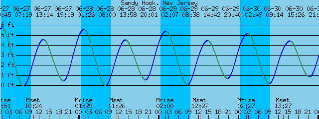
Below is the forecast of tides around Sandy Hook next week.  We will be sampling through high tide; the end of flood currents and beginning of ebb currents.  When we get strong flows of freshwater into the ocean on the ebb currents, it is relatively easy to line up sampling transects across ocean features in the vicinity of the two Seascapes. Sharp gradients form where the river of estuarine water rushes in to meet the salty, colder ocean water and those gradients are easy to see in ocean color measured with satellites, currents measured with high frequency radar, and even with the naked eye.

Each day we try to slice the dominant feature defined by a sharp gradient in temperature and/or salinity in the vacinity of each seascape in half with sampling transects that are 10 to 20 km long.  This is twice as long as the Rossby radius of deformation for our area.  One day an oceanographer will tell me what the Rossby Radius is and I'll get it. The rossby scale for the region was calculated in a paper by Yankowski on the Hudson River Plume (I think and will find the citation). As a soft scientist my dim understanding is that the size of the dominant features of circulation, usually eddies, occur at around the Rossby length scale which is determined by the strength of the currents that change with depth (slower in shallower water because of bottom friction), and by Coreolis force which changes with latitude (higher near the poles than the equator) and causes the eddies to spin (Check this explanation with a liscensed professional). Since the fish can't overcome physics, 2xs the length scale of the dominant physical features of the ocean should be the right transect length to sample the fish. We then sample at multiple depths along the transect at 5-7 stations offshore, on and inshore of the dominant ocean feature we find near the seascape. With freshwater rushing out of the estuary on the ebb tides its relatively easy to find the areas of turbulence (surface slicks, areas of with "confused" seas) along the fronts. We also have a YSI probe mounted on our research ship just below the surface. It continuously measures salinity and temperature along the ship track and we can identify the fronts between two water masses by the rapid change in either temperature or salinity in the data from that probe.